
 Canadian
Motor Simulator
Browser Compatibility: Anything modern.
Welcome to latest release of our online ebike simulator, with many new features covered in this thread. Select your motor, controller, battery, and vehicle choices then hit Simulate. Click the mouse on the graph. Fool around, and if you have any questions please read the full explanation of the features in the FAQ text below.
Tutorial Videos
Grin's Ebike Motor Simulator Tutoral: --PART 1-- Basic Overview
This is the first part of what will be a very long series on how to properly use the many the features of our popular motor simulator for ebikes:
https://ebikes.ca/tools/simulator.html
Grin's Ebike Motor Simulator Tutoral: --PART 2-- Overview of System Options
The 2nd part of the motor simulator tutorial series covers in more detail each of the various dropdown options available for setting up the simulation.
https://ebikes.ca/tools/simulator.html
Grin's Ebike Motor Simulator --PART 3-- Advanced Features (Temperature, KV, Wind Speed, Comparisons)
In Part 3 of this tutorial we go over some of the more advanced options in the simulator options:
0:00 - Intro
0:40 - Winding Temperature
1:25 - Customizing Motor KV (rpm/V)
3:15 - Seeing Effects of Wind Speed
5:00 - Comparing TWo Setups with System B
8:35 - Simulating Dual motors
10:20 - URL Encoding
11:25 - Hiding Graphs Plots
https://ebikes.ca/tools/simulator.html
How to Use the Simulator
Use the drop-down menu to choose from the list one of the hub motors that we have modeled, the battery pack, wheel size, and motor controller current limit. Then select the type of bicycle that you ride as well as the gross vehicle weight (you plus the machine) and hit "Simulate". The program will then output 4 graphical plots against your speed (in kph or mph) on the horizontal axis.
- Red Plot: The red line shows the power output of the hub motor. The power output is zero at 0 rpm, rises up to a maximum, and then falls back down to zero once the wheel is spinning at its normal unloaded speed. If the motor current is not limited by the controller in any way, then the peak power happens at between 40-50% of the motor's unloaded rpm. Otherwise, the maximum power usually coincides with the point when the controller hits the battery current limit.
- Green Plot: This is the efficiency curve for the electrical drive system. It is a ratio of the mechanical power coming out of the hub motor to the electrical power going in to the controller. This ratio accounts for losses inside the controller and the hub motor, but it does not include losses due to the internal resistance of the battery. Notice though that efficiency does not necessarily mean better range or less battery usage; a fast and powerful setup running at 80% efficiency may draw more power to cover the same distance as a slower arrangement at 75% efficiency.
- Blue Plot:The blue line can be configured to display either the torque output of the hub in Newton-meters, or the thrust of the wheel in pounds. Thrust naturally increases as you select smaller wheel sizes, while the torque of the motor is independent of wheel diameter. Torque is shown by default and increases as the wheel slows down until reaching the controller phase current limit, at which point it is at a maximum. Thrust is most convenient for estimating the climbing capacity of the vehicle, and it is what most people actually mean when they talk about 'torque'. To a first order approximation, the pounds thrust needed to overcome gravity when climbing a hill is simply weight * %grade.
- Black Plot: The black line can be configured as either the load line of the vehicle, or the % grade hill that the system will climb at steady state. The load line is the default choice, and it directly shows the amount of power necessary to move the vehicle under the selected conditions (grade hill, vehicle weight, wind speed etc.). As you increase the grade hill you are climbing, or switch to a less aerodynamic vehicle, you can see the load curve rise quite steeply at increasing speeds. The %Grade option conveniently shows in a single plot the speed at which you'd expect to climb any given grade of hill. In a glance you can see that a given setup will climb a 10% grade at 8kph, 5% grade at 19 kph, 3% at 28 kph etc. It's pretty cool and underutilized.
Cursor Bar and Text Data
By default, right after each calculation the simulator will draw a dashed vertical cursor that coincides with the point where the output power of the motor plus the human is equal to the load line of the vehicle. This is the expected steady-state cruising speed for that particular arrangement, below this speed you'll be accelerating and above this speed you will be slowing down.
You can move the cursor to any other location by clicking the graph with the left mouse button to see the numeric results anywhere elsewhere on the graph. Here you will notice that there is now an acceleration term, showing how quickly you'll be speeding up or slowing down at that point. If you have "auto" checked by the throttle slider, then on moving the cursor to a new location, the program will recomputed the simulation at a throttle setting that results in a predicted steady state speed at the cursor.
The numeric data is grouped into 3 categories:
- Graph This data here corresponds exactly to the graphical power, efficiency, torque, and load data that has already been described above. It also includes the motor RPM.
- ElectricalThis shows some of the electrical characteristics of the system at the cursor speed:
- Mtr Amps:is the phase current flowing through the windings of the hub motor. This is not the same as the current that you measure from the battery pack with a Cycle Analyst or other watt meter. At low speeds when controller is PWM current limited, it is possible for the motor current to be several times greater than the current drawn from the pack.
- Batt Power:This is the power that is being taken out of the battery pack (battery amps * battery volts), and is what you would see on the Cycle Analyst watts display. It is not the same as the actual mechanical output power of the motor, don’t confuse the two.
- Batt Amps: This is the current flowing out of the battery pack, again as would be seen by a Cycle Analyst or inline ammeter. You will notice that at low speeds the battery amps stays fixed at the controller current limit. At lower speeds still it may be fixed at the controller phase current limit. That is what a controller current limiting does.
- Batt Volts: This is the terminal battery voltage as you would see by a Cycle Analyst or Voltmeter. As you move the cursor to lower speeds where more current is drawn from the battery, you'll the voltage on the battery pack sag due to internal resistance.
- PerformanceThe performance table shows the vehicle characteristics at the cursor speed:
- Acceleration:This shows the instantaneous expected acceleration or deceleration of the vehicle at the particular cursor location. If the motor output power and human power exceeds the load power of the vehicle, it will accelerate. If the motor power is less, it will decelerate. The units will be in either mph/sec or kph/sec.
- Consumption: This is the Wh/km or Wh/mi as you would expect to see on the Cycle Analyst for the energy consumption of the vehicle. It is a direct measure of how much battery energy you use per distance traveled.
- Range:This is the predicted distance you could achieve from a full charge on the selected battery pack. It is based on the available battery capacity and not the nominal amp-hours. So for instance the "12Ah" SLA option has an actual capacity of just under 8Ah due to the Peukert effect.
- Overheat In: This is a prediction on how long it would take the motor to overheat (reach 150oC) from the starting temperature of the simulation, based on a comprehensive thermal motor model taking into account both the motor RPM and passing air velocity. If the motor has not had been thermally characterized in our wind tunnel, then it will say "Not Modeled" instead.
- Final Temp:This is a prediction of the motor core temperature after running for 2 hours at the current conditions for phase current, rpm, and velocity. The text will appear red if the final temp is over 150 oC. It is very common to run hub motors for short times at loads that cannot be sustained continuously, most steep hills are over in a matter of minutes rather than hours.
Using the Throttle Slider
Many people overlook the fact that there is a throttle slider and only bother looking at the full throttle output, and come to incorrect conclusions related to 'efficiency' and 'sweet spot'. If you want to see how a system behaves at slower speeds, which is achieved in practice by backing off on the throttle, then move the throttle slider to less than 100% or choose the "auto" checkbox and then click on the graph at the lower speed you want to simulate.
Comparing Two Systems
If you would like to compare two setups side by side, then the link "Open System B->" will pull out a 2nd table from which you can select an entirely different system and have both plots show up together on the same graph. A second set of numeric data shows up in the tables as well. There will be two cursors, left clinking will position the system 'A' cursor and right clicking will position system 'B' cursor.
Dual Motor Systems
With System 'B' open, you also have the option to add the output power of the two setups (A and B) to simulate a dual motor drive on a single vehicle. Appropriate fields will be greyed out, so you only have one vehicle to model. Note as well that the two systems each require their own battery pack, it does not model dual drives pulling energy from a single battery.
Hiding Plots
It is possible to hide any of the plotted data to make for a cleaner graph. The circle beside each plot title in the legend is also a radio button, so you can click the dot to show or hide the associated line. This is particularly useful when you are comparing two systems and otherwise would have 8 plots to deal with on the graph.
Entering Custom Values
We have provided dropdown selection for a range of typical battery packs, vehicle types, and motor controllers. At the bottom of each of these menus is a 'custom' option that brings a pop-up menu if you would like to simulate with different components.
- Custom Battery:This enables you to simulate a system with a battery type or voltage not listed in the dropdown.
- V: This is the open circuit and not the nominal battery voltage. So for instance, a nominal 36V LiFePO4 pack sits at about (12 cells * 3.3V/cell) = 39.6V, and not 36V.
- Ω: This is the internal battery resistance and is an important detail, and the simulator can misbehave if it is left at zero. If you do not know the resistance of your pack, then try to find this info from the manufacturer or vendor. Any respectable supplier would know or be able to get this detail. Lacking that, you can get the data by observing the voltage of your system under load. For instance, if a battery is showing 49V at rest, and 44V when you draw 25A at full throttle, then the battery resistance is approximated by ΔV/ΔA = (V49-44V)/(25A) = 0.2 Ω.
- Ah: This is the actual output capacity of the pack in amp-hours, and is used only for the expected range calculation. If you are modeling a lead acid battery, the actual capacity is usually about 30-40% less than the nominal capacity due to the Peukert effect.
- Custom Controller:Controllers are currently modeled as having a battery current limit, phase current limit, and your choice of a voltage throttle (typical ebike controller), a torque throttle (common with field oriented controllers), or an amps throttle (commonly done via a V3 Cycle Analyst).
- Battery Current Limit: This is the controller current limit, and reflects the maximum current that the controller will draw from the battery before automatically entering a PWM current limited mode.
- Phase Current Limit: This is the maximum current that the controller will output to the controller, and is generally in place to protect against damaging the controller mosfets at low speeds. Many ebike controllers do not have any phase current limiting and just rely on the battery current limits, but for those that do it is usually somewhere between 2-3 times the battery current limit.
- Effective Resistance Ω: This is the combined resistance of both the mosfets and the phase leads going from the controller to the hub motor. It can be estimated from the resistance of 2 mosfets (one high side, one low side) plus the controller->motor lead resistance based on the wire gauge. For instance, a controller with 10mΩ mosfets and a 6 foot 14g motor lead wire would have a resistance of (2*10mΩ + 2*6 feet* 2.52Ω/foot) = 50 mΩ, or 0.05Ω.
- Custom Motor:The ability to enter custom motors is a new feature for advanced users only. Details are explained in the pop-up fields.
- Custom Vehicle:Here is where you can model the rolling and aerodynamic characteristics of your particular vehicle. We recommend checking out the speed and power calculator at https://kreuzotter.de/english/espeed.htmfor more details on typical drag coefficients for bicycles.
- CdA: This is the effective frontal area for the vehicle, which can range from 0.2 for a fairly streamlined recumbent up to 0.8 for a wide upright mountain bike with a puffy jacket. All aerodynamic calculations are done assuming sea level elevation and ambient temperatures.
- Cr: This is the rolling drag coefficient of the vehicle wheels. Bike tires range from about 0.004 for a high pressure road slick, up to 0.012 for a low pressure knobby wheel.
Simulator FAQ
With the direct drive motors this is easy. Once you move the cursor passed the unloaded motor speed, the graphs for motor torque and battery current both go negative, allowing you to see how much power will be required to turn the motor and how much electrical current and power would be generated. Even though the graphs don't display far into the negative region, you can use the numeric tables to see generated power deep into regen mode.
With the geared motors (eZee and BMC), we have modeled the freewheeling behaviour of the motor. Above the unloaded speed the motor is assumed to spin at the unloaded RPM regardless of the wheel RPM, and you cannot see the regen behaviour that would be possible if either the freewheel was locked or the motor was spinning in reverse.
The inflection point that you see occurs when the motor controller hits the current limit. At speeds above this point, the current from the battery gradually declines until it reaches 0 amps at the unloaded rpm (where the graph outputs intersect). At speeds slower than the inflection point, the motor controller regulates the power to the hub, restricting battery current draw to the motor controller current limit (20A, for example). In this region, from 0 rpm up to the inflection point, there is constant power input into the motor rather than a constant voltage, and so the nature of the curves is different.
That is because even though the battery current is limited by the controller, the current through the motor is not. It is the motor current, not the battery current, that determines the torque output of the hub motor. When there is no Pulse-Width-Modulation (PWM) going on in the motor controller (full throttle and moving fast enough that the battery current is under the motor controller current limit) then the amps flowing out of the battery is effectively the same as the amps flowing through the motor. But when the controller is doing PWM, then the current through the motor is higher than the battery current by the inverse of the PWM duty cycle.
That is because of the inductance of the motor windings. At each commutation event, current in the phase winding that was just disconnected needs to decay through a freewheeling diode in the controller. While this current decays, it is still present in the motor leads and generating torque even though it is not drawing any current from the battery pack. So the net result is a somewhat higher phase current than battery current, even at full duty cycle. This effect is most pronounced in high speed geared motors (e.g. BMC, eZee), somewhat less noticeable in high pole count direct drive hubs (e.g. Nine Continent, Clyte H series), and barely discernable in low pole count direct drive motors (eg. Clyte 400 and 5300 series).
While we appreciate the level of interest that has been shown in the simulator by other businesses who would like to have a copy of it on their site, the answer is that no, we are currently not interested in licensing this online software. It is first and foremost a tool that we have made freely available via our website to the ebike community.
Doing a full characterization of a hub motor takes a lot of our time and is done at our discretion.
Simulator Details
The old simulator was based on the following circuit model for a battery-powered permanent magnet motor and controller setup:
- VOCis the open circuit battery voltage.
- Rbattis the first order internal resistance of the battery.
- Ibattis the current draw from the battery pack.
- Controlleris assumed to be a single quadrant (non-regen) controller, with the indicated input and output equations.
- D is the PWM duty cycle, which can range from 0 to 1. This value is generally equal to the throttle setting, but that can be over-ridden to keep Ibattat the specified current limit.
- Imotoris the current through the motor windings.
- Rmotoris the winding resistance of the motor.
- Kis the motor constant, in Nm/A or V/(Rad/sec).
- w is the wheel speed in radians per second.
The actual model in SimulatorV2 is substantially more complicated, taking into account the commutations that happen on a regular basis as a function of the speed and number of poles of the hub motor, and determining the resulting current waveforms that are produced when this is applied to the inductive motor windings.

The power is calculated simply as this output torque times wheel speed:
The efficiency is calculated from the input power to the controller divided by the output power (it does not take into account the losses internal to the battery pack):
Finally, the road speed is calculated based on wheel size. The simulator also correctly shows the regen currents and negative power when the wheel is spinning faster than the unloaded voltage, so the axis go slightly in the negative region to show this.
Accuracy and Limitations
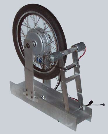
The parameter values that are chosen for the motor model are based on directly measured data that we have compiled from tests using a custom built dynamometer made for the task.
Our original 2005 dynamo setup pictured above was limited to a maximum loading of about 5 N-m, but we have since built two newer devices, one of which allows for continuous load testing of the hub motors of over 50 N-m of torque. This has enabled us to verify the mathematical model above to the measured output performance with a high degree of accuracy and over a wide speed and power range.
Credits: Motor modeling, algorithms, and GUI design by Justin Lemire-Elmore. The back-end web programming to make this into an awesome online app was started by Zev Thompson back in 2006 and significantly updated in more recent years by the hard work of Michael Vass and Adam Hynek.